Temporal data and waves | Berken Utku Demirel

Contrastive learning

Contrastive learning is a framework for self-supervised representation learning, where the objective is to bring semantically similar samples closer in the latent space while pushing dissimilar ones apart. Since the labels are not available during the self-supervised learning, contrastive learning relies on carefully designed data augmentations to generate similar samples, with the choice of augmentations playing a critical role in overall performance [1].

Importance of data augmentation

In contrastive learning, augmentation is crucial for extracting good representations from unlabeled data. Research has demonstrated that poorly tailored augmentations can significantly decrease the performance of the models on downstream tasks. Some papers claimed that effective data augmentations preserve task-relevant information while discarding nuisance variables [2-3]. One of the theoretical works regarding the contrastive learning [3] suggested that augmentations introduce a controlled chaos that helps align intra-class samples by emphasizing their similarities. For instance, two distinct cars might appear more alike if both images are cropped to focus on the wheels, highlighting common features while downplaying differences. This raises a natural question: how can one preserve task-relevant information in temporal data while simultaneously generating diverse samples through augmentations?

Augmentation for time series

To preserve task-relevant information, it is essential to first establish a rigorous method for quantifying information. For this purpose, we rely on one of the fundamental measures in information theory: the Signal-to-Noise Ratio (SNR).

\[\mathcal{I}(\mathbf{y}; \mathbf{x}) \propto \int_{f^*}^{} S_{x}(f) \mathbin{/} \int_{-\infty}^{\infty} S_{x}(f) \hspace{2mm} \text{where} \hspace{2mm} S_{x}(f) = \lim_{N\to\infty} \frac{1}{2N} \left| \sum_{n=-N}^{N} x_n e^{-j2\pi f n} \right|^2,\]

where $S_x(f)$ denotes the power spectral density of the signal $\mathbf{x}$, and $f^*$ represents the frequency ranges carrying task-relevant class-specific information. Almost all augmentations in temporal data do not concern about the SNR. Augmentation in time series differs from image or text augmentation due to its inherent structure. Traditional methods like resampling or random noise addition fail to retain task-relevant information and SNR. Mixup [4], a method that linearly interpolates two samples for augmentation, retains information from both samples. The augmented sample, $\mathbf{x^+}$ incorporates features from the original anchor sample, $\mathbf{x}$, and a randomly chosen sample, $\mathbf{\tilde{x}}$, as in the equation below.

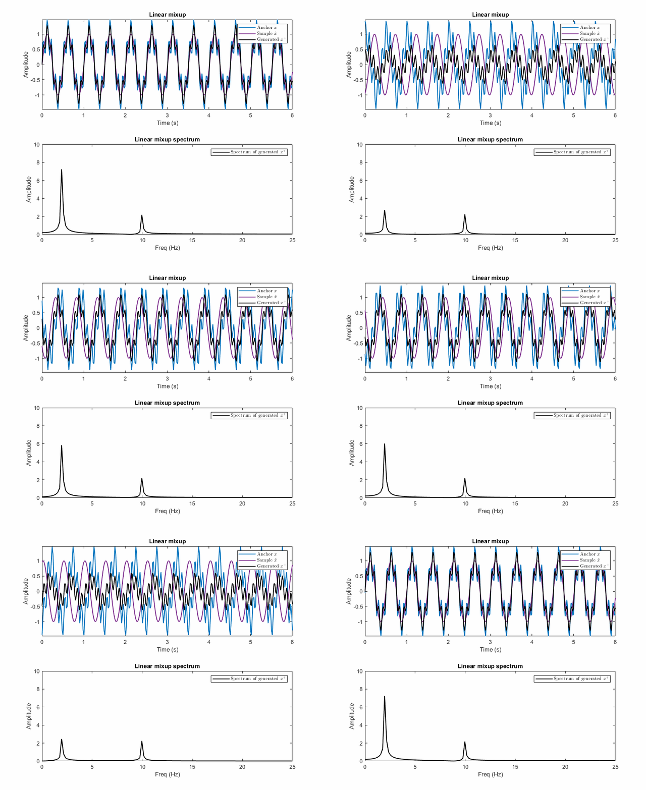
\[\mathbf{x^+} = \lambda \mathbf{x} + (1-\lambda) \mathbf{\tilde{x}}\]

For temporal data, the linear mixup method may lead to destructive outcomes rather than preserving task-relevant information. Specifically, this augmentation can potentially destruct the critical task-specific details. This behavior stems from the phenomenon of destructive interference, where two waves interact, and result a combined wave with diminished amplitude.

Destructive Mixup:
There exist $ \lambda \sim \text{Beta}(\alpha, \alpha) $ or $ \lambda \sim U(\beta, 1.0) $ with high values of $ \beta $, such that when linear mixup is used, the lower bound of the mutual information for the augmented sample distribution decreases to zero:

\[ 0 \leq \mathcal{I}(\mathbf{y}; \mathbf{x^+}) < \mathcal{I}(\mathbf{y}; \mathbf{x^*}), \] where $ \mathbf{x^*} $ is the optimal sample that only carries *task-relevant information*, \[ \mathbf{x^+} = \lambda \mathbf{x} + (1-\lambda) \mathbf{\tilde{x}}, \quad \text{and} \quad \int_{f^*}^{} S_{x^*}(f) = \int_{-\infty}^{\infty} S_{x^*}(f). \]

Interference phenomena in mixing two waves stems from the phase difference between coherent signals. To prevent this, we perform the linear mixup for the magnitude of each sinusoidal. However, for the phase, we take a different approach and bring the phase components of the two coherent signals together by adding a small value to the anchor’s phase in the direction of the other sample to prevent destructive interference. The mixup operation performs the linear interpolation of features, however, interpolation of two complex variables can result in a complex variable whose phase and magnitude are completely different/far away from those two, i.e., mixup can be destructive extrapolation. Therefore, the phase of two sinusoidal can be interpolated by first calculating the shortest phase difference between the two coherent waves for all frequencies, denoted as $\Delta \Theta$, as in equation below.

$$\begin{align} \begin{split} \theta &\equiv [\mathnormal{P} (\boldsymbol{\mathrm{x}}) - \mathnormal{P} (\boldsymbol{\mathrm{\tilde{x}}})] \text{mod}{(2\pi)}\\ \Delta\Theta &= \begin{cases} \theta - 2\pi, & \text{if } \theta > \pi \\ \theta, & \text{otherwise} \end{cases} \end{split} \end{align}$$

Where $A(\mathbf{x^+})$ is the linearly interpolated amplitude, and $P(\mathbf{x^+})$ is the phase of all sinusoidals for the generated sample $\mathbf{x^+}$.

Based on the calculated phase difference between two samples, we perform the mixup operation to generate diverse positive samples, such that the phase and magnitude of augmented instances are interpolated properly according to the anchor sample $\boldsymbol{\mathrm{x}}$, without causing any destructive interference.

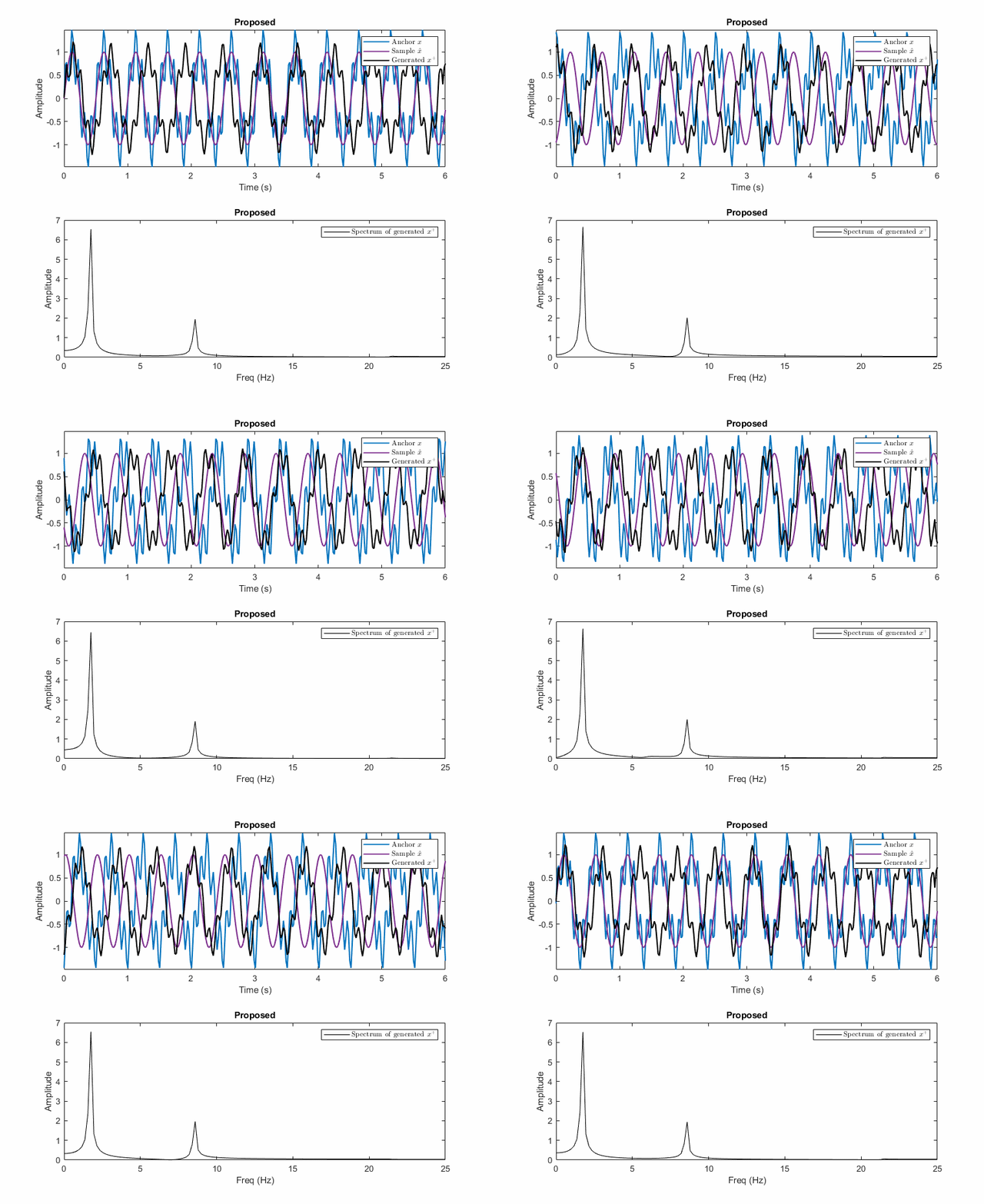
\[\begin{equation}\label{eq:proposed_aug} \begin{gathered} \mathbf{x^+} = \mathcal{F}^{-1} (\mathnormal{A} (\boldsymbol{\mathrm{x^+}}) \angle \mathnormal{P} (\boldsymbol{\mathrm{x^+}})) \hspace{3mm} \text{where} \hspace{2mm} \mathnormal{A} (\boldsymbol{\mathrm{x^+}}) = \lambda_A \mathnormal{A} (\boldsymbol{\mathrm{x}}) + (1-\lambda_A) \mathnormal{A} (\boldsymbol{\tilde{\mathrm{x}}}) \hspace{2mm} \text{and} \\ \mathnormal{P} (\boldsymbol{\mathrm{x^+}}) = \begin{cases} \mathnormal{P} (\boldsymbol{\mathrm{x}}) - |\Delta \Theta| * (1-\lambda_P), & \text{if } \Delta \Theta > 0 \\ \mathnormal{P} (\boldsymbol{\mathrm{x}}) + |\Delta \Theta| * (1-\lambda_P), & \text{otherwise} \end{cases} \end{gathered} \end{equation}\]

Examples of this destructive and the proposed mixup is illustrated with an example below. In the example, the anchor has two frequencies [f1: 2Hz, f2: 10Hz] and the other sample has only one at 2Hz, e.g., 2Hz carries information while the anchor has noise at 10Hz. The possible generated samples are plotted when the phase of the 2Hz sinusoidal changes between $-\pi$ and $\pi$.

Sum of two sinusoidal in time and frequency domain using linear mixup

Sum of two sinusoidal in time and frequency domain using the proposed method

As seen in these figures, the presented method prevents the destructive mixup by operating in the frequency domain separately for the magnitude and phase of each sinusoidal.

Does it work always?

Although the presented method prevents destructive inference when two waveforms are summed up, it assumes the signals are quasi-periodic which can be described as the observed signals exhibiting periodicity on a small scale, while being unpredictable on a larger scale. Otherwise, the performance of the augmentation decreases as the frequency of the waveforms change over time (non-stationary), where we also observed this in our experiments.

References

1. A simple framework for contrastive learning of visual representations. In Proceedings of the 37th International Conference on Machine Learning, ICML 2020.

2. What makes for good views for contrastive learning? In Proceedings of the 34th International Conference on Neural Information Processing Systems. NeurIPS 2020.

3. Chaos is a Ladder: A New Theoretical Understanding of Contrastive Learning via Augmentation Overlap. International Conference on Learning Representations. ICLR 2022.

4. mixup: Beyond Empirical Risk Minimization. International Conference on Learning Representations. ICLR 2018.